Quarterly Report
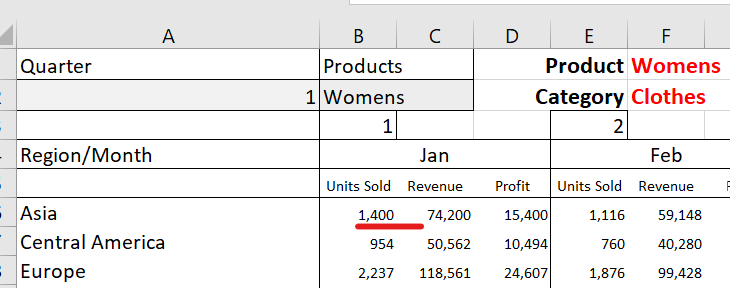
The quarterly report shows monthly figures for regions, 3 months at a time. The report shows total units sold, revenue and profit for every month of the quarter and the totals for the quarter. At the left end of the report, full-year results of 2019 are included for comparison.
The report allows the analysis of the results for each product and all products.
The formulas are in the same format with the report tables, but they include more parameters.
Cell B6 =SUM((_RE=$A6)*(_MO=B$3)*IF($B$2=”All”,1,(_PN=$B$2))*_SU)
(_RE=$A6) filters the region column for the region stated in cell A6
(_MO=B$3) filters the month column for the month stated in cell B3
(_PN=$B$2) filters for the product stated in Cell B2, if the value in cell B2 equals to all returns 1 and the product filter is not applied
_SU takes the total for the filtered context
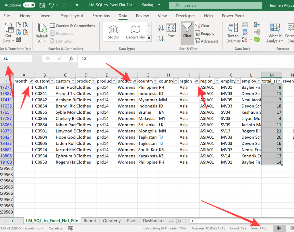
You can go to data sheet ‘LM_SQL_to_Excel_Flat_File’, put filter to the data, apply the region/month/product filters mentioned above and take the total of total_sales (total units sold) column, which will show the same result of the formula above.
There is a drop-down list at cell A2, the list has numbers 1 to 4, corresponding to the quarters of the year.
This drop-down list feeds into the month part, (_MO=B$3), of the array formula in cell B6. The if statements in cells B3, E3 and H3 reads the number in the drop-down list and return the month number to the array formula.
Cell B3 =IF(A2=1,1,IF(A2=2,4,IF(A2=3,7,IF(A2=4,10,0)))) – as the list shows 1st quarter, the formula returns 1. This cell is for the first month of the quarter (Q) so the values it get for 1st Q =1, 2nd Q = 4, 3rd Q = 7 and 4th Q = 10.
Below there is an explanation for creating a drop-down list.
The second drop-down list is on cell B2 shows the list of the products. This drop-down list feeds into the month part, (_PN=$B$2), of the array formula in cell B6.
To create this list, we copy the product list from the report sheet cells Y2:Y27 to quarterly sheet cells U2:U27. We add All for all products to cell U28.
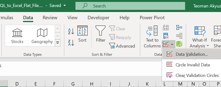
Select cell B2, in Quarterly sheet where we will set the drop-down list. Then from Data menu Data Validation tab select Data Validation.
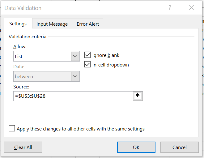
In the Data Validation dialogue, Settings tab select list and set the source to $U$3:$U$28, press OK.
Test the list choosing the products from the list.
Cell F3 shows the product (both versions), and F4 shows the related product category (Excel 365 version).
To display related product category, we use the new XLOOKUP formula (only Excel 365).
XLOOKUP(F1,_PN,_PCAT) – searches the product stated in F1 in database _PN (product) column, returns the corresponding value on _PCAT (product category) column for the first value found in _PN column.
F4 =IF(B2=”All”, ,XLOOKUP(F1,_PN,_PCAT)) – Displays XLOOKUP result if cell B2 does not show “All”.
When you play with the drop-down lists you will see that Excel is freezing for short periods, even with powerful computers it is much slower now. Excel calculates all formulas in the workbook when a single calculation is triggered, and as we add more calculations and they get more complex Excel will be slower.
Now analysis of The Report is complete and you can go forward with The Pivot.