The Report
There are a lot of ways to pull insights from data in Excel. Especially to answer our simple questions, pivot tables are the fastest and most efficient way. We will anyway start with formulas because this is the real power of Excel for bespoke reporting.
Now open the ‘LM_SQL_to_Excel_Flat_File.csv’ in Excel and save it as .xlsx file. Create a sheet and name it ‘report’.
In the report sheet, we start with the questions.
1. Monthly sales totals of Lead Merchants (units sold, revenue, profit)
2. Report regional sales figures (units sold, revenue, profit)
3. Sales by product (units sold, revenue, profit)
4. List top 10 countries by revenue
5. Customer profitability: top 100 customers by profit
6. Employee performance: report top 5 employees who made the highest profits
There are good practices working with a large amount of data in Excel. An important one of them is parsing the data by naming its columns and referring these columns with their names in formulas. A good practice for naming is to start with a _ for each name and put short but easy to keep in mind names to each column. Select all data in the column you want to name and write the name in the name box. For customer names, we chose column C cells 2 to 229.561 and input name ‘_CUNA’ or find a better name that suits you and press enter.

Our names are:
| Column | Names | Reference |
| month | _MO | =LM_SQL_to_Excel_Flat_File!$A$2:$A$229561 |
| customer_id | _CU | =LM_SQL_to_Excel_Flat_File!$B$2:$B$229561 |
| customer_name | _CUNA | =LM_SQL_to_Excel_Flat_File!$C$2:$C$229561 |
| product_category | _PCAT | =LM_SQL_to_Excel_Flat_File!$D$2:$D$229561 |
| product_id | _PID | =LM_SQL_to_Excel_Flat_File!$E$2:$E$229561 |
| product | _PN | =LM_SQL_to_Excel_Flat_File!$F$2:$F$229561 |
| country | _CN | =LM_SQL_to_Excel_Flat_File!$G$2:$G$229561 |
| country_id | _CNID | =LM_SQL_to_Excel_Flat_File!$H$2:$H$229561 |
| region | _RE | =LM_SQL_to_Excel_Flat_File!$I$2:$I$229561 |
| region_id | _REID | =LM_SQL_to_Excel_Flat_File!$J$2:$J$229561 |
| employee_id | _EID | =LM_SQL_to_Excel_Flat_File!$K$2:$K$229561 |
| employee_name | _ENA | =LM_SQL_to_Excel_Flat_File!$L$2:$L$229561 |
| total_sales | _SU | =LM_SQL_to_Excel_Flat_File!$M$2:$M$229561 |
| revenue | _SR | =LM_SQL_to_Excel_Flat_File!$N$2:$N$229561 |
| _cost | _SC | =LM_SQL_to_Excel_Flat_File!$O$2:$O$229561 |
| stock | _ST | =LM_SQL_to_Excel_Flat_File!$P$2:$P$229561 |
You can view, add or edit names in name manager:

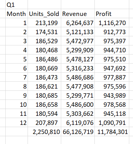
Q1. Monthly sales totals of Lead Merchants (units sold, revenue, profit)
We create a table on cells B2 to E14. Name the row cells B2 to E2 as Month, Units_Sold, Revenue, Profit. Name the column cells B2 to B14 from 1 to 12 representing months.
There are a lot of ways that you can create these formulas. I prefer good old array formulas.
Formula –
Cell C3=SUM((_MO=B3)*_SU)
Cell D3=SUM((_MO=B3)*_SR)
Cell E3{ =SUM((_MO=B3)*(_SR-_SC))} – The curly brackets in the last formula
are the old way of entering array formulas, which is not necessary anymore.
Press shift+ctrl+enter (CSE) to enter the array formula.
Select cells C3 to E3 and copy until/including C14 to E14.
Finally, enter SUM to get subtotals at cells C15 to E15.
Q2. Report regional sales figures (units sold, revenue, profit)
We will create a table from cells G2 to J9 to present region figures.
Name row 2 as Regions, Units_Sold, Revenue, Profit and column G as the name of the regions.
Now how do we find the list of the regions (or products, customers, countries, employees for other questions)? We do not have a separate file for each of these like we had in SQL, and we have to pull them from the huge flat file.
There are a few ways, but luckily Microsoft released new array formulas in September 2019, which makes life a lot easier in such cases.
Find the list of regions
Formula –
Cell V3=UNIQUE(_RE) – this is a new array formula, it spills over the cells
below and gives a list of unique values in the referenced name _RE, regions
column of the flat table (currently unique function works only Excel 365
version, download the file without UNIQUE function below).

Note that we only entered the formula to Cell V3 and it spilt over to Cell V9 and populated the whole list. Examine these cells; in V3 there is the formula we enter, and we can delete and edit it. In other cells, there are the spilt formulas in shaded grey, which means you can neither delete nor edit them. They are dependent on the formula entered in cell V3.
Now follow the procedure we did in Q1; copy the region names to cells J3 to J9, enter the below formulas to cells from H3 to J3 and copy these formulas up to cells H9 to J9 and take subtotals.
Formula –
Cell H3 =SUM((_RE=G3)*_SU)
Cell I3 =SUM((_RE=G3)*_SR)
Cell J3 =SUM((_RE=G3)*(_SR-_SC))

Q3. Sales by product (units sold, revenue, profit)
Formula –
Cell Y3=UNIQUE(_PN) - A list of all products
Create a table from cells L2 to O27 and apply the same procedure in the previous question with the below formulas to present product figures
Formula –
Cell M3 =SUM((_PN=L3)*_SU)
Cell N3 =SUM((_PN=L3)*_SR)
Cell O3 =SUM((_PN=L3)*(_SR-_SC))

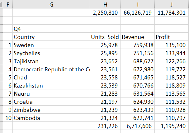
Q4. List top 10 countries by revenue
Formula –
Cell AB3=UNIQUE(_CN) - A list of all countries
Step 1-
Create a table from cells G13 to J198 and apply the same procedure in the previous question with the below formulas to present country figures
Formula –
Cell H14 =SUM((_CN=G14)*_SU)
Cell I14 =SUM((_CN=G14)*_SR)
Cell J14 =SUM((_CN=G14)*(_SR-_SC))
Step 2-
Now we have a list of 185 countries, and we only have to report the top 10 by revenue. The best way to achieve this is a pivot table, but we are keen to do this with formulas at the report work.
Select the table (cells G13:J198), sort Z to A (largest to smallest) by revenue and delete the cells below row 23. Take totals to row 24 for countries table.
Note that we could set a filter to this table and filter the top 10 countries. But unlike pivot tables, the filter hides all contents in a row, not only filtered table, which is a problem when data from other tables or formulas exist in the same row.
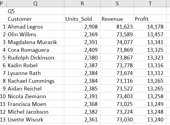
Q5. Customer profitability: top 100 customers by profit
Formula –
Cell AE3=UNIQUE(_CUNA)                  - A list of all customers (a magical
 954-row list pulled out from 229.561-row dataset by one simple formula)
Step 1-
Create a table from cells Q2 to T956 and apply the same procedure in the previous question with the below formulas to present customer figures
Formula –
Cell R3 =SUM((_CUNA=Q3)*_SU)
Cell S3 =SUM((_CUNA=Q3)*_SR)
Cell T3 =SUM((_CUNA=Q3)*(_SR-_SC))
Step 2-
Go on with the same procedure as with Q4 and delete after 100 customers.
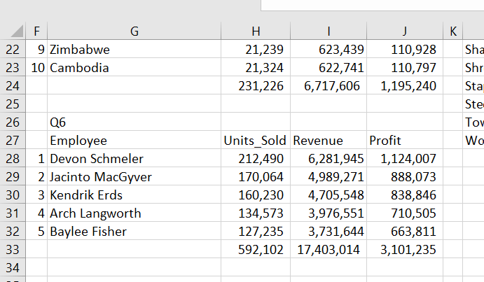
Q6. Employee performance: report top 5 employees who made the highest profits
Formula –
Cell AH3 =UNIQUE(_ENA) - A list of all employees
Step 1-
Create a table from cells G27 to J48 and apply the same procedure in the previous question with the below formulas to present employee figures
Formula –
Cell H28 =SUM((_ENA=G28)*_SU)
Cell I28 =SUM((_ENA=G28)*_SR)
Cell J28 =SUM((_ENA=G28)*(_SR-_SC))
Step 2-
Go on with the same procedure as with Q4 and delete after 5 employees.
With the above tables, all questions are answered. The reporting in real life is much more complex than preparing these tables. To show the power of Excel on bespoke reporting and to give a flavour of Excel’s versatility in performing calculations and pulling valuable insights from data, we move forward with a second report sheet, Quarterly. This sheet shows quarterly results for each region, in comparison with full-year figures and allows analysis per product.
The quarterly report also presents a simple use of the new XLOOKUP formula. Follow the link to see an explanation of this sheet.
Next is the Pivot.