Power BI Desktop
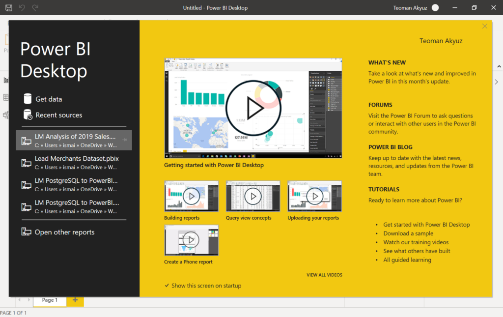
Open the Power BI (PBI) desktop, sign in, and the program starts with the below dialogue box.
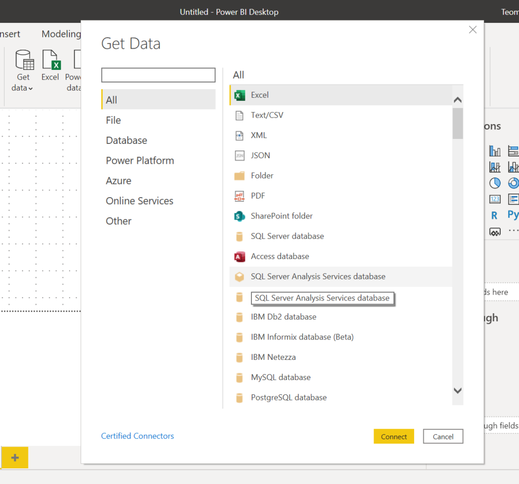
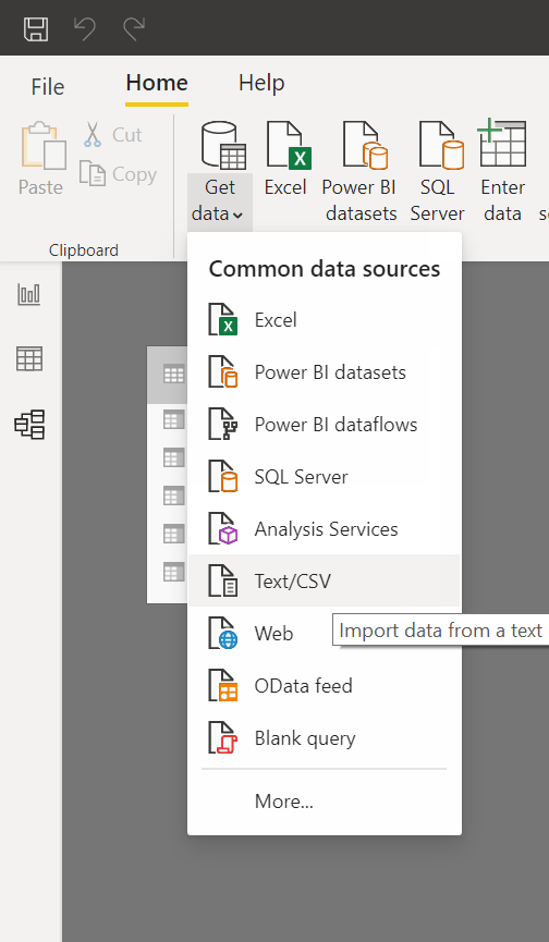
Press get data and get the data dialogue box opens. Here you can see there is a very long list of data/container types you can load to Power BI. Scroll down the list to see the list. An important feature of PBI is you can load data from different resources and add different types of data to your data model.
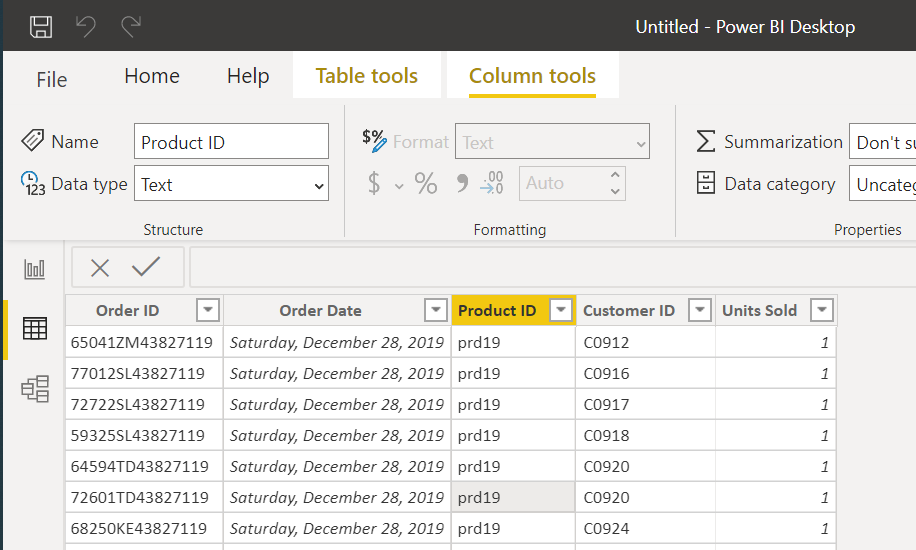
We have LM Sales database tables in CSV format. Select Text/CSV, find the orders table from the load dialogue, and you’ll reach a new dialogue box showing the columns of the orders table along with some data and specifications of the table.
PBI recognised the colımn names in the first row, if not we have to transform data to add column headers.
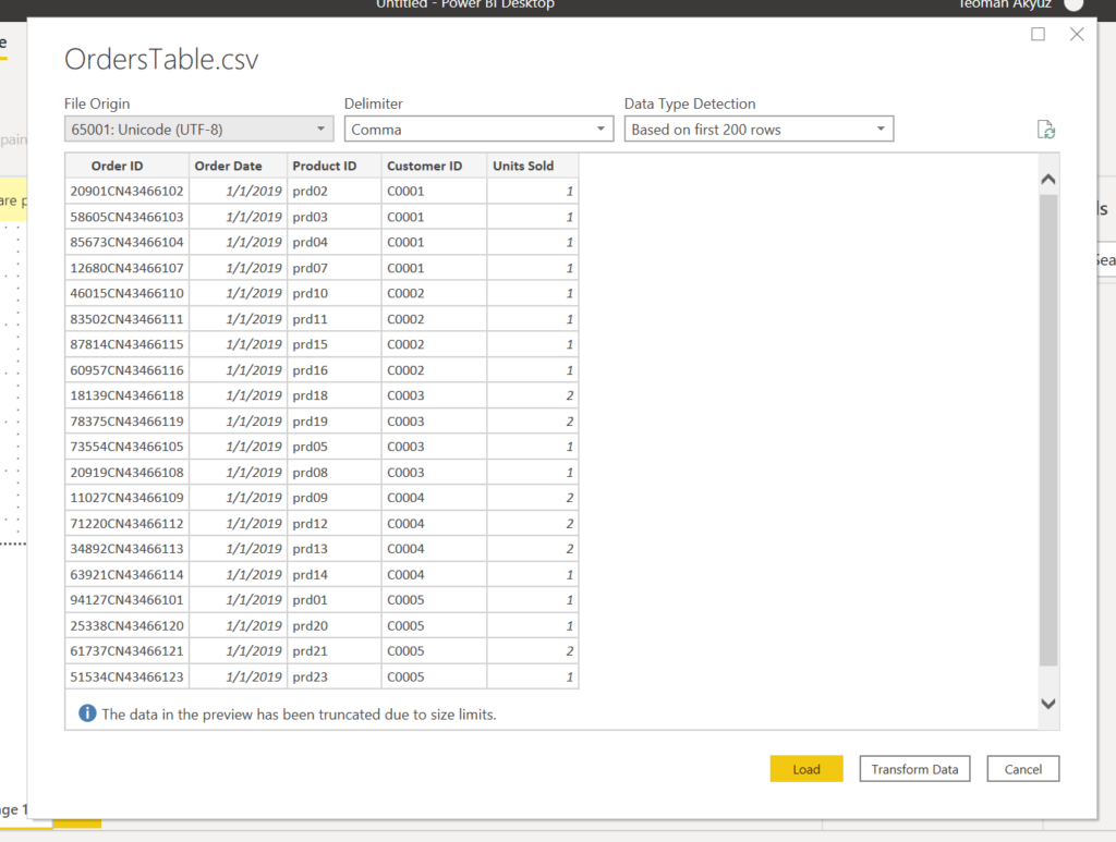
Below you see 3 buttons, Load takes us directly to PBI; in case we need to make some adjustments to data such as column headers, fill empty cells, change data type etc. we have to press Transform Data, which will take us to Power Query (PQ).
Press load, orders table will be loaded to PBI, and you will land in PBI Report view.
There are 3 views on the PBI desktop, which you can see at the far left of the window, below the ribbon.
The top button shows the Report View, where the results and visualisation are presented on the PBI desktop.
The middle button brings to the Data View. This is similar to Power Pivot Data View. In this view, you can see the tables and make operations on the tables, such as adding columns or measures necessary to perform the analysis.
The last button is for the Model View, which has the same functionality as the Power Pivot Diagram View. You can define table connections and set up database relationships.
The current view, the Report View, is empty, as we have not prepared any reports or visuals yet. We go to the Data View to examine the table we just loaded.
Let’s have a look also Model View and then go on with loading other tables.
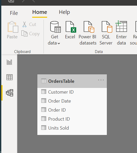
Now load the other 4 tables of the database.
Under the Home, menu select the Get Data tab and select Text/CSV to load the country table.
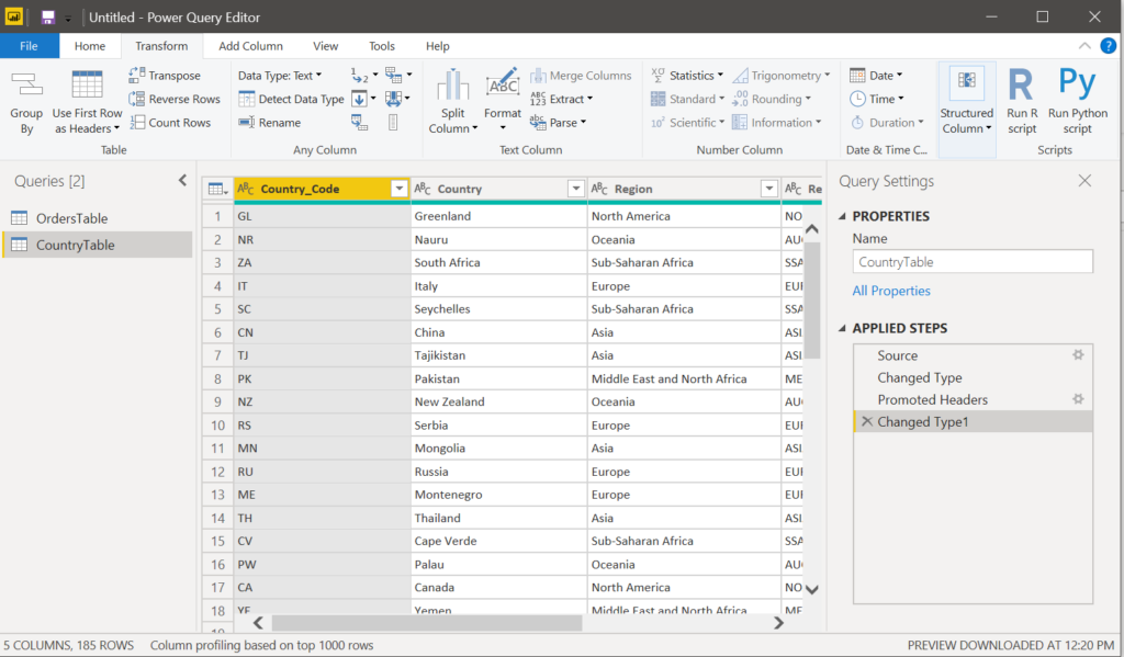
While loading the country table, it is possible that PBI does not recognise the first row as column headers. You have to go to the Power Query to set the first rows as table headers.
In the PQ window under the Transform menu select ‘Use First Row as Headers’ which will correct the headers.
Under the Home menu press Close & Apply; this will take you to Data View in PBI.
Go on and load other tables.
In the model view, you can see 5 tables. PBI has already established the relationships between tables. We have to check if they are aligned with our data model.
Go on to arrange the tables in the best visual order.
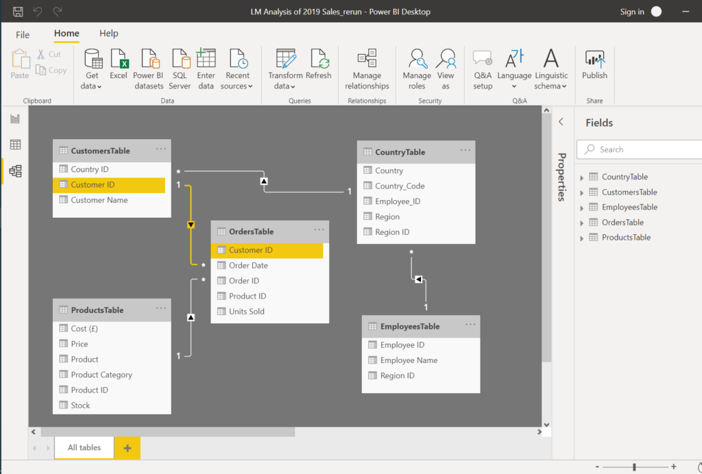
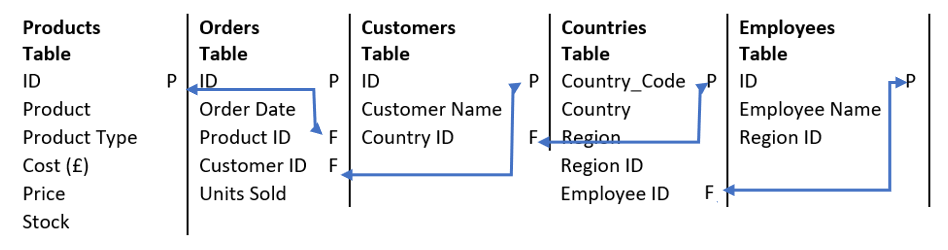
Click any line of an established relationship to check which fields are used for connections, and use the table below to set up the data model with connecting Primary Keys to Foreign Keys.
This is now a good time to save the file we are working on.
On the right of the window, there is the Fields pane in all Views. This pane shows all tables and their columns. You can do some edits on the tables and columns in Model view but we will go to Data View and work on the tables there.
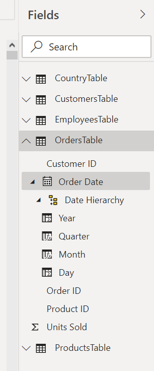
In the data view, we can add columns and measures. We will not add a month column because PBI creates a date hierarchy when it recognises date columns. This enables analysis in desired granularity, daily, monthly, quarterly and yearly.
In the data view under the fields pane, you can see the OrdersTable Order Date column date hierarchy.
We will go on and add the measures we added in Power Pivot.
On the fields pane right-click on the OrdersTable title, you can see the operations you can do over the tables. Select New Measure from the drop-down list (or press the New Measure button on the Table Tools ribbon).
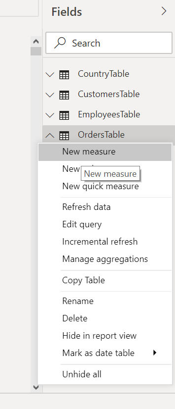
A bar similar to Excel Formula Bar will appear in the window, stating 1 Measure1.
The 1 at the beginning means you are in the first line; you can line multiple lines to execute at one go.
Change the measure name as Cost and write the DAX formula, press enter.
Cost = SUMX(OrdersTable, [Units Sold] * RELATED(ProductsTable[Cost (£)]))
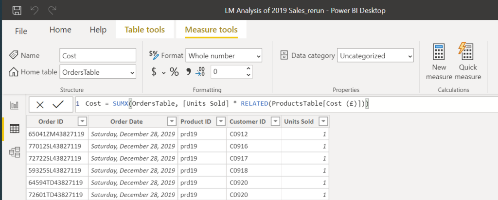
Recognise that this is the same formula that we wrote in Power Pivot in DAX language.
In the Fields pane under the orders table, a new column, ‘Cost’ will appear.
Add formulas for Revenue and Profit.
Revenue = SUMX(OrdersTable, [Units Sold] * RELATED(ProductsTable[Price]))
Profit = [Revenue] - [Cost]
We have now these measures, Cost, Revenue, Profit which you can see under fields pane in all views.
This is all we will do with the tables, and we will now create the Report and answer the below questions.